Lecture 8: Huffman Coding

Attribution

Much of the content from these notes is taken directly or adapted from the notes of the same course taught by Dr. Andrew Forney available at forns.lmu.build.

Introduction

As a reminder, greedy algorithms are those that explore some search space by always taking the next “best” looking action.

We have seen some examples of greedy algorithms already:

• Greedy approaches to the Changemaker problem, wherein the largest denomination possible is taken at each step.
• Greedy search prioritization in which the evaluation function is $f(n)=h(n)$ (i.e., only considering the next “best looking” action, not the ones that also consider the past / path cost $g(n)$).

In many of problems we have seen so far, greedy algorithms don’t perform as well as other algorithms. This isn’t always the case, however, and today we will see an example where a greedy algorithm is optimal.

Motivating Example

Consider the following 300 x 300 colored boxes: one that’s all white, one that’s all blue, and one that’s a gradient between them.

Question

Which of the images above do you think will have the largest file size? Why?

The white and blue squares will have roughly the same size, while the gradient square will be much larger. This is because the gradient square has many unique colors, while the white and blue squares have only a few unique colors.

In the most naive case of storing an image, we could record every pixel’s $(x,y)$ coordinate and the RGB value of that pixel in a 2D array. RGB values for colors are encoded as a spectrum in which each of the RGB color channels is some value between $[0,255]$ for a total of $256\times 256\times 256$ different possible combinations.

This is why we often denote colors by their hexadecimal code like #FF0000 because 6 hex digits provide $256\times 256\times 256$ color combinations!

Question

How many bytes does a single RGB value / hex code take to store?

A single RGB value / hex code takes 3 bytes to store. This is because $16\times 16=256=2^8$, meaning that every 2 hex digits create one byte (one RGB value). Thus, if an $N\times M$ image would require $N\times M\times 3$ bytes to store.

This is wasteful, though! Not all images have all $256^3$ different colors.

Data Compression

Data compression is the process of encoding data using fewer bits than the original representation.

Question

Why is data compression important and what are some of its applications?

Data compression is important because memory and bandwidth are limited resources, so maximizing them can be vital.

Some example applications of data compression include:

• Image compression: finding concise ways of storing images is important lest we burn tons of memory in wasted space.
• Zip archives: finding ways to compress groups of files in a portable, concise format is vital for transmission and in some cases, security.
• Text transmission: ever played a real-time multiplayer game? Bandwidth can only transfer so many bytes at a time, so finding concise ways of transmitting vital information can improve on lag.

Important

To make use of any compressed data (image or otherwise) we must first decompress it into its original format, or something close to it.

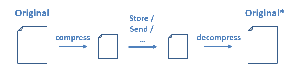
Note the asterisk on the decompressed version of the file. The decompressed version may be either an exact replica or something close to it depending on the type of compression used.

There are two different categories of compression algorithms based on guarantees about the decompressed file:

• Lossy algorithms provide approximations of the original and are typically used for images and video in which perfect fidelity is not necessary, but speed or transmission size is of highest priority.
• Lossless algorithms provide perfect recreations of the original once decompressed.

Approach to Data Compression

Question

Is it possible to have a Universal Compression Algorithm (UCA) that, given any data, can compress it further?

No, it is not possible to have a Universal Compression Algorithm. If that were possible, then we could take any original file, compress it, then compress that compressed version etc. until we were left with 1 bit!

Question

How do you think we can decrease the size of an image file (think about the 3-box example from above)?

We may be able to decrease the size of an image file by changing how we represent commonly occurring colors. In other words, why use three bytes to store every pixel’s color if an image only uses two colors? For the two-color example, we could instead use a single bit to represent each pixel’s color (e.g., 0 for white and 1 for blue)!

More generally, our goal with compression will be to take the most common data components and assign them the smallest representation (least number of bits).

Compression Goals

Rather than start with the more complex problem of image compression, we’ll see the same techniques applied to text compression.

Text Encoding

Consider the extended-ASCII encoding by which every character corresponds to an 8-bit (1 byte) representation:

An encoding schema defines the rules for translating information in one format into another. In the cases of character encodings, we are mapping character symbols in text to their bytecodes (i.e., the bits that are stored in memory and can then be translated to the letters we see on the screen).

There are also different encodings for images and pretty much any file or information you store on a computer. To go the more analog route, Morse Code is another type of encoding in which tones / different-length symbols translate to letters.

ASCII encoding is a type of fixed-length code, since every character takes up the same amount of space. For instance, the character ‘A’ is represented by the bytecode 0100 0001, while the character ’!’ is represented by the bytecode 0010 0001:

Decimal	Bytecode	Character
65	0100 0001	A
33	0010 0001	!

Question

Suppose we are storing some text file in which some characters appear much more frequently than others; why might the above be wasteful? Can you suggest an approach to do so?

Just as in the 3-box example, using a fixed-length encoding like ASCII can be wasteful if some characters appear much more frequently than others and if not all characters are used.

Question

What might be a better approach to encoding text, then?

We could use a variable-length encoding that assigns shorter codes to more frequently occurring characters and longer codes to less frequently occurring characters.

Consider the following string: AAAABBBCCD. Using extended ASCII, it would take $10\times 8$ bits to represent these 10 letters. Perhaps we can do better by observing that ‘A’ appears most frequently, so we could represent it using something short like 0, and ‘B’ (which appears second-most) as something like 10.

For example, we could use the following encoding:

Bytecode	Character
0	A
1	B
10	C
11	D

Question

What is wrong with the encoding above?

The above encoding is problematic because it is ambiguous. For example, the code for ‘A’ (0) is a prefix of the code for ‘C’ (10).

Question

What property / guarantee should our encoding make so that the above never happens?

We need to ensure that no whole code is a prefix of another code in the system.

Prefix Codes (also known as Prefix-Free or Huffman Codes) are those in which no whole code is a prefix of another code in the system. Although this is a limiting property in the amount of compression we can do, it is also a necessary one for being lossless.

To recap, we want to create an encoding schema that:

• Compresses some corpus of text to require fewer bits to represent it than it takes in its original format.
• Performs this compression by finding a variable-length, prefix-free encoding that is influenced by the rarity of each character in the corpus.
• Is lossless such that the original string can be reconstructed with perfect accuracy during decompression.

Huffman Coding - Compression

Huffman Coding is a procedure for finding a prefix-free, lossless, variable-length compression code for some data (image, text, or otherwise) by encoding the most common data components with the most concise representations.

The steps of Huffman Coding Compression are:

Let’s find the Huffman Encoding of the following string: ACADACBABE.

Step 1: Find Character Frequencies

Since we want to use the most concise encoding for the most common characters in the string, the first step is to find the distribution over each character in the corpus.

This is a simple task:

• Tally each instance of each character.
• Divide the final counts by the total string length to find their distribution.

In our example string ACADACBABE, we have $N=10$ characters over which:

Character	Count	Probability
A	4	0.40
B	2	0.20
C	2	0.20
D	1	0.10
E	1	0.10

Question

Which character do we want to have the smallest code (i.e., represented with the fewest bits)?

A, since it is the most common character.

Step 2: Find Encoding Map

With this distribution in hand, we now need to find a mapping of each character to the bit-code used to represent it.

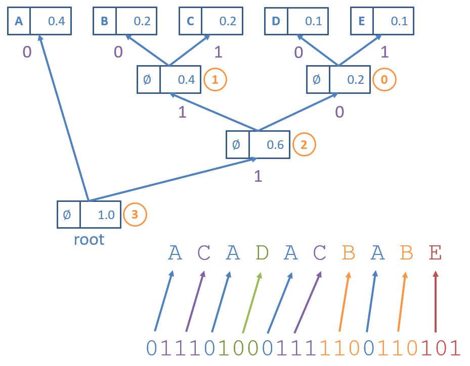
The Huffman Encoding Map is generated as a binary trie (another word for a Prefix Tree, AKA a Huffman Trie) in which:

• Nodes have at most 2 children and is labeled with the frequency of characters in their subtrees.
• Leaves exist for each character being encoded.
• Edges represent bits in each character’s encoding, with each non-leaf having a zeroChild (with an edge labeled 0) and a oneChild (with an edge labeled 1).

Construction of the Huffman Trie proceeds as follows:

for each character to encode:
    create leaf node and add to priority queue
while more than 1 node in queue:
    remove 2 smallest probability/count nodes from priority queue
    create new parent node of these 2 removed with sum of their probabilities
    enqueue new parent
last remaining node in priority queue is the root

Some notes on the Huffman Trie above:

• Each leaf node has a character and priority / frequency associated with it, but inner nodes just have the priority (no character).
• The circled, orange numbers indicate the order in which parents were generated for the children from the priority queue.
• The Encoding Map is generated from the Huffman Trie by tracing the path from the root to the character’s corresponding leaf, which can be created simply by using a depth-first traversal.

Question

Is the code generated using the Huffman Trie going to be optimal? i.e., will it reduce the code length of each character optimally according to its probability?

Yes! A proof by induction works here: no subtree that occurs more frequently will have a parent added before a subtree that occurs less frequently.

Question

Is the code generated using the Huffman Trie going to be prefix-free? Why or why not?

Yes! Observe that every branch induces a new prefix.

Question

Is the encoding generated using the Huffman Trie unique?

No, the encoding generated using the Huffman Trie is not guaranteed to be unique — whenever two characters have the same frequency, their encoding can be swapped. For instance, we could have also generated the Huffman Trie below:

Question

Does it matter which Huffman Trie we use in terms of optimal compression?

No, as we will now see, the compression rate is the same for both Huffman Tries.

Step 3: Compress Corpus Using Map

With the Encoding Maps created from the previous step, finding the compressed version of the corpus is easy. To encode a text corpus using a Huffman Encoding Map, simply replace each character with its corresponding code in the map.

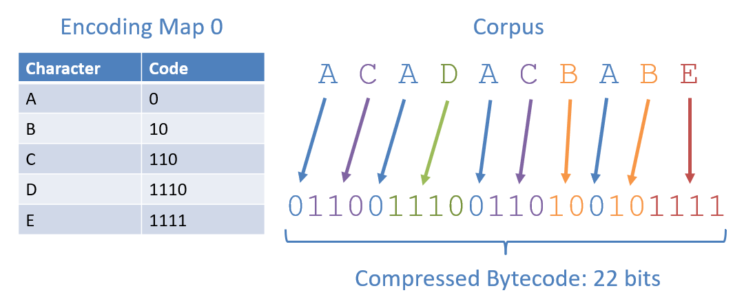
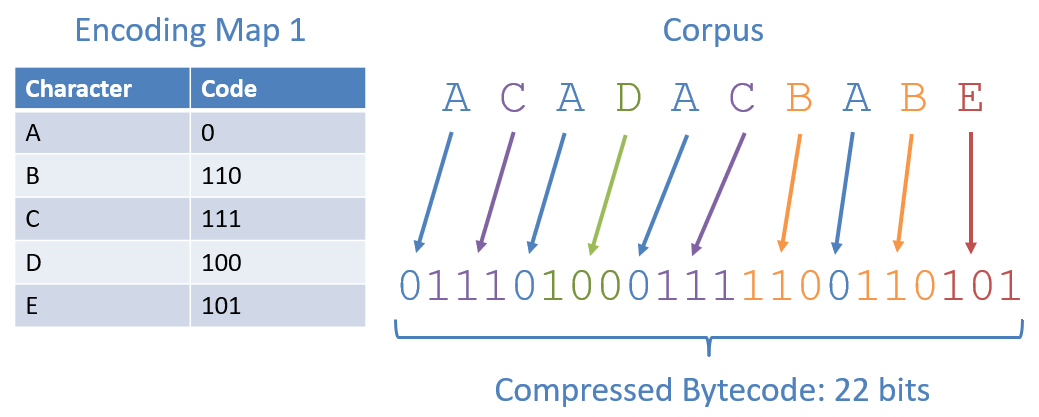
Some notes from the figures above:

• Both encoding maps (although different codes) lead to the same compression rate.
• The compressed bitstring associated with the Huffman Encoding is 22 bits, compared to the 80 bits required by Extended-ASCII to encode this corpus.

Huffman Coding - Decompression

Now that we have compressed something, let’s see how to get it back!

Decompressing a Huffman Coded string works in reverse, taking a Huffman Coded bitstring and reconstructing the original. When in possession of the Huffman Trie and compressed bitstring, the decompression process is trivial:

• Start at the root of the trie and the first bit in the bitstring.
• Follow the zeroChild reference whenever a 0 is encountered in the bitstring, and the oneChild reference when a 1 is encountered.
• Add the letter corresponding to a leaf node to the output whenever the above traversal hits a leaf.
• Begin again at the root for the next letter to decompress.

Consider how to decompress the bitstring 0101 0110 0101 1000 1001 11 generated using the Huffman Trie shown earlier:

Question

How do we guarantee that this decompression process will uniquely translate back to the original?

By generating a Huffman Trie that is a prefix-free encoding, there is a unique path from the root to each character.

Question

Is there a rather large assumption (with regards to decompression) that we’re making with the above?

Yes! We’re assuming that, upon decompression, we have access to the Huffman Trie that generated the code. This may be a bit presumptuous: consider the case wherein we are compressing some corpus of text to transmit to another computer via some network:

Question

How might we ensure that the decompression process always has access to the compression encoding map?

We can include the Huffman Trie as part of the bitstring’s header. Our encoded bitstring then consists of two components:

• The header, containing meta-data about the file and a means of recovering the encoding map.
• The content, which is what needs to be decoded.

Question

Why would it be insufficient to send the characters and their frequencies in the header as a means of recovering the encoding map?

Since frequencies / Huffman Codings are not unique for a particular corpus, we may not be able to recover the exact Huffman Trie that was used to compress it. For instance, in our two encoding maps from the previous section, 110 is the code for ‘C’ in Map 0 but ‘D’ in Map 1. Since both Map 0 and 1 are the results of valid Huffman Tries on the same corpus, the frequencies of each character alone will not suffice in telling us which it was that was sent: Map 0 or 1.

Encoding the Huffman Trie

A simple approach to converting the Huffman Trie into the bitstring’s header is to perform a preorder traversal of the trie:

encodeTrie(Node n):
    if n is a leaf:
        add 1 to header
        add decompressed character to header
    else:
        add 0 to header
        encodeTrie(n.zeroChild)
        encodeTrie(n.oneChild)

Consider encoding the Huffman Trie corresponding to Encoding Map 1:

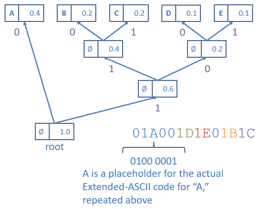
Some things to note about this encoding strategy:

• We use 0 as a flag to indicate an internal node and 1 as a flag to indicate a leaf node.
• When a leaf node is encountered, by “add decompressed character to header,” we mean that (if the original corpus was encoded in Extended-ASCII) we would add the bytecode for the character that the leaf represents directly following the flagged 1 bit.

Decoding the Huffman Trie

To reconstruct the Huffman Trie from its header encoded bitstring, we simply walk back the preorder traversal:

• Left nodes are always visited before right.
• Leaf nodes are always first flagged by a 1 bit.
• Internal nodes are always flagged by a 0 bit, meaning we recurse.

Consider recovering the Trie associated with the following header:

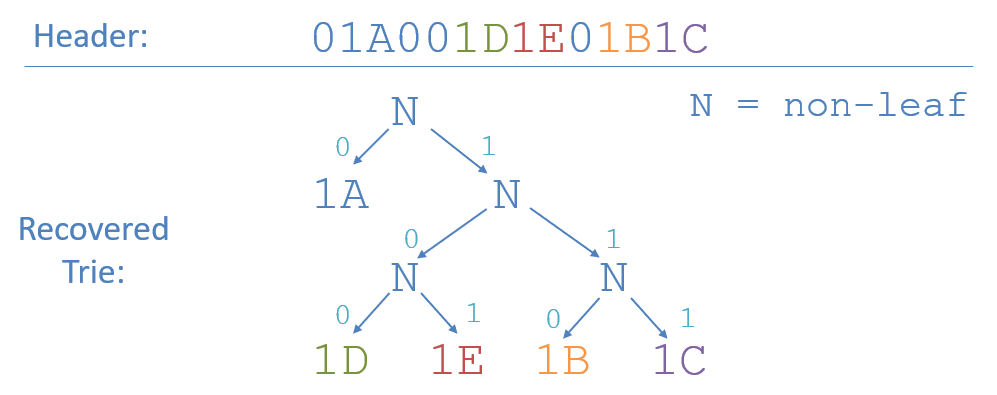
No ambiguity, the full Huffman Trie is at our fingertips, and we can continue to decode the message at our leisure!

Conclusion

In this lecture, we learned about Huffman Coding, a technique for finding a prefix-free, lossless, variable-length compression code for some data. We saw how to compress a corpus of text using Huffman Coding and how to decompress it. We also discussed how to include the Huffman Trie as part of the bitstring’s header to ensure that the decompression process always has access to the compression encoding map.

To test your understanding, consider the following practice problems:

1. Encode the Huffman Trie associated with Encoding Map 0 from the examples above.
2. Decode the following message! If you’ve been following along this far, you must be awesome!
   • Header: 01A01B01C01D1E
   • Content: 1110 1111 0 1110