Lecture 3: Adversarial Search and Pruning

Note

Much of the content from these notes is taken directly or adapted from the notes of the same course taught by Dr. Andrew Forney available at forns.lmu.build.

Introduction

So far, we have been considering search problems in which a single agent is trying to find a path to a goal. In these problems, the agent is the only entity in the environment whose actions we need to consider. These types of problems are known as classical search problems. In this lecture, we will consider a different type of search problem in which there are multiple agents in the environment.

Unlike classical search problems, in which the agent’s actions are determined solely by the environment, in multi-agent environments, the agent’s actions are influenced by the actions of other agents. There are many interesting problems in which agents act cooperatively in an environment, such as drone coordination and triangulation. In this lecture, however, we will focus on adversarial search problems, in which agents’ goals are in conflict. These types of problems are often referred to as games or adversarial search problems.

Question

Consider the maze path-finding problem we discussed in the previous lecture, but with a twist: there are two agents in the maze and one agent is trying to block the other agent from reaching the goal. Will our previous approaches to search work in this scenario?

No! Our previous approaches planned a sequence of actions from the initial state to a goal, but that plan can be interrupted by another agent acting to prevent it. We’ll need to make our agents reactive to adversaries!

Games have been of intense interest in the development of AI. Chess-playing bots, for example, have been a metric for the success of AI design. Modern AI agents are now competing in even more complex games that require a great deal of planning and foresight (e.g., Google’s advances in bots that play the game of Go).

Canonical Games

In AI and game theory, the most commonly analyzed games are somewhat basic and have the following properties:

• Two players (adversaries), $P_1$ and $P_2$
• Turn-based, such that $P_1$ acts first, then $P_2$, then $P_1$ again, and so on
• Perfect information, such that the game state is fully observable and no chance or probability is involved
• Constant-sum, such that one player wins, the other loses, or both tie

Question

Can you think of any games that match these qualities?

There are also many games that have variations of these properties. For example, card games are instances of games with imperfect information, since each agent cannot see the other’s hand.

Question

Can you think of any games that are variations of the canonical game properties?

As we’ve previously seen, even small variations in problem formulation can lead to drastic changes in the environment, which in turn changes the approaches we use to find solutions. Next, we’ll see an example of a canonical game and start to develop the tools that will help us find solutions.

Adversarial Problems

Let’s start by looking at a motivating example game and then discuss how we can formalize the problem.

The Game of Nim

The game of Nim has a rich history with many variants, but we’ll look at a simple variant to motivate our discussion. In this variant of the game, there are $N$ stones in a pool. On each turn, players can remove $1$, $2$, or $3$ stones from the pool. The player who removes the last stone is the winner.

Question

Try playing a game of Nim with $N=12$ stones against a partner!

Now that we’ve seen the game in action, let’s formalize its components and see how we can create an agent that plays it intelligently.

Adversarial Problem Formalization

We can formalize an adversarial search problem by specifying six qualities:

1. State: Contains all game-specific features that change during the game.

2. Player: Represents whose turn it is to act in a given state. $\text{player}(state)\in \{p_1,p_2,\dots \}$

3. Actions: The set of all actions available from a given state. $\text{actions}(state)=\{a_1,a_2,\dots \}$

4. Transitions: How some action transforms the current state to the next state. $\text{transition}(state,action)=\text{nextState}$

5. Terminal tests: Determines if the state ends the game. $\text{terminal}(state)\in \{T,F\}$

6. Utility functions: Returns a numerical score for a terminal state from the perspective of a given player. $\text{utility}(state,player)=u$ Generally speaking, for two terminal states $s_1$ and $s_2$, if $\text{utility}(s_1,p)\ge \text{utility}(s_2,p)$, then $s_1$ is more desirable to player $p$ than $s_2$.

In constant-sum games (also called zero-sum games), the sum of utilities for all terminal states (summing across all players) is the same value.

${\sum }_{p\in \text{Players}}\text{utility}(s_1,p)={\sum }_{p\in \text{Players}}\text{utility}(s_2,p)\forall s_1,s_2\in \{s:\text{terminal}(s)\}$

For example, a reasonable utility score for Nim is to have, for some state $s_1$ in which $p_1$ wins:

$\text{utility}(s_1,p_1)=1;\text{utility}(s_1,p_2)=0$

Note how this is a constant-sum utility function, because for every terminal state, the sum of utilities is $1$.

Let us now see how we can use this information to develop a plan of attack!

Search for Games

Let’s start by considering how we solved search problems in the classical domain and see how we can apply similar strategies to adversarial search problems.

Question

How did we explore possible solution paths in classical search problems? What structure did we use, and can we apply that here?

We used search trees! We can try to apply that to our adversarial search problem, except that every other state along a path will be decided by our opponent. We call this structure a game tree, which:

• Shows all possible moves from all players to the game’s terminal states
• Contains utility scores for each player at each of the game’s terminal states

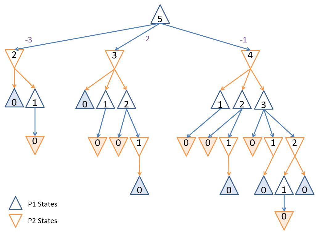Game tree for a small game of Nim with $N=5$.

Question

In classical search, we had the notion of goals, which were terminal states that also satisfied the problem. In adversarial search, we have terminal states, but what is different about them compared to classical search?

Some terminal states are goals for one player (i.e., they meet some optimization criteria), while others are goals for another player. To distinguish which states are good for which player, we can score them with a utility function. Since this is a zero-sum problem (more accurately, a constant-sum problem) in which a single player either loses (e.g., utility = 0) or wins (e.g., utility = 1), we can score our terminal states from the perspective of our agent appropriately.

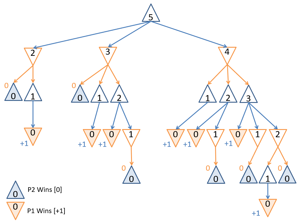Game tree for a small game of Nim with $N=5$, scored from the perspective of the first player.

The figure above shows the game tree scored from the perspective of the first player (i.e., the root). The utility scores for each terminal state (leaf node) is $0$ if the first player loses (there are no stones left for the first player to remove), and $1$ if the first player wins (there are no stones left for the second player to remove).

Utility Scores

Now let’s consider how we can use these utility scores to plan the best action for our agent.

Question

Since we have to worry about our opponent acting against our goals, we should plan for the worst and then adapt. What is the worst-case scenario for our opponent’s action policy?

The worst-case scenario is that our opponent acts optimally (i.e., they always choose the best option available to them). Under this assumption, we want to act optimally assuming that our opponent does as well.

In cases where our opponent does act optimally, we are not surprised; in those when they do not, we will do even better than projected! All that’s left is to characterize how an optimal opponent will act, and then how we can respond.

Question

If our opponent is always trying to win, is always acting optimally, and an opponent win means that we get a score of $0$, then what are our opponent’s actions trying to do to our score?

Minimize it! Note that this is a consequence of Nim being a constant-sum game, because an opponent trying to maximize their score is the same as them trying to minimize ours. Conversely, if our opponent is trying to minimize our score, then we’re trying to maximize it. Thus, in a constant-sum game tree, opponent states can be characterized as Min Nodes and our states as Max Nodes.

Mini-Max Mechanics

Mini-max search is a search strategy that, given a current state and a problem specification, will determine the next optimal action for our agent. Formally:

$\text{minimax}(state,problem)=\text{bestActionFromState}$

Question

In classical search, our solutions were an ordered sequence of actions. Why does Mini-Max search return only a single action from the current state?

Because our opponent chooses its own actions based on our actions, we cannot formulate an entire plan independently of our opponent’s actions. We must first see how our opponent acts after we choose our optimal action from the current state.

The basic steps of Mini-Max are as follows:

1. Look ahead at (and score using the utility function) possible terminal states from the actions available to us
2. Consider what paths our (optimally acting) opponents will take and our optimally acting response
3. Determine the best path according to the best score for our agent

Question

Can you think of any algorithms that can help guide our agent to the optimal solution, given the game tree with utility scores at the terminal states?

The prescription of Mini-Max search suggests that we “score” each non-terminal state and then make a decision that maximizes that score. We can associate a score with each node such that:

• Every terminal node is scored via its utility
• Every Min Node attains the minimum utility/minimax score of its children
• Every Max Node attains the maximum utility/minimax score of its children

The optimal action (for Max = our agent) from the current state is thus the one that maximizes the score at the root.

Question

Given that we need to score the terminal nodes first to obtain any minimax scores, what kind of search strategy is Mini-Max a variant of?

Depth-first search, since we must consider the deepest nodes (the terminal states) before scoring the others.

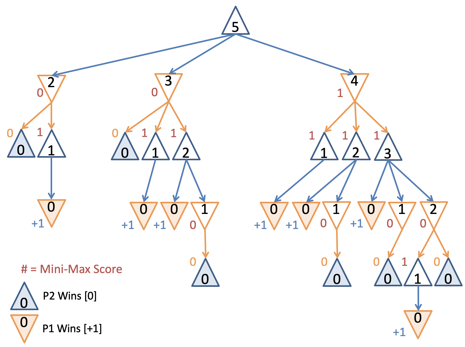Game tree for a small game of Nim with $N=5$, scored from the perspective of the first player.

The figure above shows the game tree with each intermediary state scored from the perspective of the first player.

Given the Mini-Max scores at each node, the action that the maximizing player should take at the root is to remove just $1$ stone from the pool. And there you have it! Mini-Max Search in a nutshell.

Question

What are some issues with the game-tree approach we’ve discussed so far?

We had to label every single intermediate state with a score. If the game tree is large, this could be prohibitively expensive computationally!

α-β Pruning

Let’s start by trying to optimize the number of nodes we need to expand in our game tree to perform Mini-Max search. Consider the following stage in our Mini-Max game tree generation using the depth-first strategy:

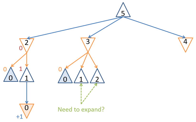Partially expanded game tree for a small game of Nim with $N=5$. Do we need to expand the rightmost branch?

Question

Once we have explored the subtree from the $-3$ action at the root, and are considering the $-2$ action, do we need to expand other children of the root’s $3$ child as soon as we’ve discovered that a winning move for Min exists?

No! As soon as we see that the $-2$ action would lead to an opponent’s win as well, we need not look any further — that action will lead to an equivalently scored outcome as one we previously explored.

Consider the $1$ child of the root’s $3$ node: this would lead to a victory for Max, but is not a move that the Min player would ever take, given that there exists a winning action for Min from the parent (and so the $1$ node should be ignored). This is an example of a scenario in which the Mini-Max search need not completely populate the game tree. Pruning is a technique in search in which we never expand a node in the search tree that we know will never lead to a solution or one with a higher quality than what we’ve already found. This technique can lead to savings in computational and space complexity, especially for larger game trees.

The $\alpha$-$\beta$ Pruning variant of Mini-Max search stops exploring an action’s sub-tree as soon as it is determined that the action is equally- or worse-scored than some previously explored sub-tree. Let’s step through some intuitions for how to approach an implementation of the above!

Question

What kind of search pattern should we use to explore the game tree?

Depth-first search (using a stack frontier) is the best choice since we need to bubble-up terminal node utilities to obtain each non-leaf’s minimax score.

Question

What does Mini-Max Search return from a given state rooting the game tree and how does it do this?

The best action to take from the state at the root. It does this by comparing the minimax scores of all of the root’s children and selecting the action that led to the highest.

Question

Since we only need the game tree for deciding a single action (i.e., do not need to remember paths like in classical search), what other depth-first programming paradigm could be used to explore the game tree without needing to create any nodes at all?

Recursion! We can implement Mini-Max search’s exploration of the game tree recursively and do not need to create the game tree — we can instead just pass the theoretical Mini-Max node fields as arguments to a recursive call.

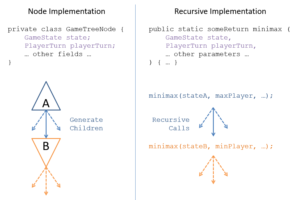Recursion-based implementation of Mini-Max search.

Given that Mini-Max search can be implemented recursively, we can obtain the Mini-Max scores from any child nodes through the recursive call’s return value; call this value $v_X$ for a returned value from child $X$.

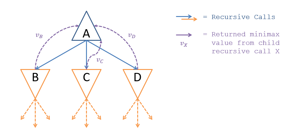Recursion-based implementation of Mini-Max search with α-β pruning.

We prune the tree by tracking two values at each node representing the best and worst scores we’ve found in previously-explored paths. Call these two values tracked at each “node” $\alpha ,\beta$ such that:

• $\alpha$: The smallest score already encountered from a previously-explored path (i.e., the worst the max agent can do elsewhere)
• $\beta$: The largest score already encountered from a previously-explored path (i.e., the best the max agent can do elsewhere)

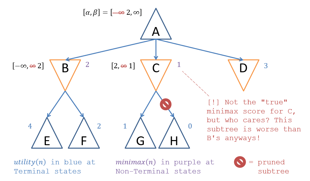
Consider the example where the values of $[\alpha ,\beta ]$ at min-node $A$ are $[3,6]$ and the values that would be returned by Mini-Max for each of $A$‘s children are $v_B=4,v_C=2,v_D=1$.

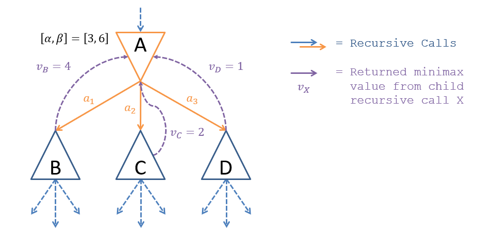Example of α-β pruning.

Question

Look at the example in the figure above. After exploring which of the subtrees $\{B,C,D\}$ would we be able to prune the others?

After exploring subtree $C$, we would find a move that’s worse ($v_C=2$) than the worst we can do elsewhere ($\alpha =3$), which already makes it less desirable than what we’ve found beforehand and thus need not explore subsequent subtrees. In this case, we would thus stop exploring $A$‘s children as soon as the recursive call to $C$ returns, and return the lowest value seen so far as $v_A$ (since $2$ is now the min of any explored children). Note that this might look funny because $v_D=1$, which is even worse than $v_C=2$, but since we never explored the $D$-subtree (since we didn’t need to), we just return the min of what we did explore (it won’t matter).

Example of α-β pruning.

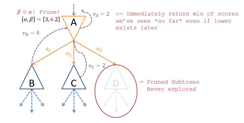
This insight characterizes our final intuition before we look at the actual procedure: $\alpha$-$\beta$ pruning won’t always deliver the correct Mini-Max value from a node (like above), but it also doesn’t need to, because if subtrees are ignored, it’s because the scores there won’t change our existing decision.

Example of α-β pruning.

Notably in the figure above, as soon as we reach terminal $G$, we would prune the other of $C$‘s subtrees ($H$) because a score of $1$ is already worse than $B$‘s previously-explored subtree’s score of $2$ — and it could only get worse! In fact, it does, as $H$‘s score is $0$, but we don’t care and just return the minimum of $C$‘s child scores that we’ve seen thus far, knowing that we’re not going to use its results.

Proceduralizing α-β Pruning

The implementation of $\alpha$-$\beta$ pruning is as follows:

• Each “node” (i.e., recursive call) record-keeps its own values of $\alpha ,\beta$ that are maintained as follows:
  • The root begins with $[\alpha ,\beta ]=[-\infty ,\infty ]$ since no exploration has been done at the start.
  • Each child node’s $[\alpha ,\beta ]$ are inherited from their parents’ to start.
• While exploring a node’s subtrees recursively:
  • A node’s $\alpha$ is updated only if it is a Max node when a child’s score $v>\alpha$ (we’ve found better than we minimally had elsewhere).
  • A node’s $\beta$ is updated only on Min nodes when a child’s score $v<\beta$ (we’ve found worse than what we maximally had elsewhere).

The values of $[\alpha ,\beta ]$ establish a range of utilities that represents the Mini-Max scores that still carry some useful information — if that range ever shrinks to nothing (or less than nothing), then there is no point in continuing to explore! Formally, this makes our pruning criteria such that whenever $\beta \le \alpha$, the range of useful values is empty, and thus we can return from that recursive call.

The following pseudocode of the $\alpha$-$\beta$ pruning algorithm is from Wikipedia:

function alphabeta(node, α, β, turn)
    if node is a terminal node
        return the utility score of node
    if turn == MAX
        v = -∞
        for each child of node
            v = max(v, alphabeta(child, α, β, MIN))
            α = max(α, v)
            if β ≤ α
                break
        return v
    else
        v = ∞
        for each child of node
            v = min(v, alphabeta(child, α, β, MAX))
            β = min(β, v)
            if β ≤ α
                break
        return v

Additionally, assuming we’re starting with the maximizing player’s turn, we would start the ball rolling with the call:

$\text{alphabeta}(\text{root},-\infty ,\infty ,\text{MAX})$

Tip

This project has great interactive α-β pruning for you to practice on! You’ll need to download the repo first, then launch the index.html file.

As an exercise, try to fill in the blanks in several examples of the above. Also, apply $\alpha$-$\beta$ pruning to our original Nim $N=5$ problem (solution in the figure below).

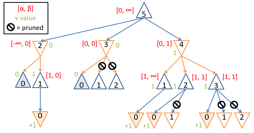Game tree for a small game of Nim with $N=5$, scored from the perspective of the first player, with α-β pruning.

Asymptotic Performance

Let’s spend a brief minute discussing the computational merits of $\alpha$-$\beta$ Pruning… in particular: just how effective is it? Consider again our tree metrics of $b$, the tree’s branching factor, and $d$, the depth of the game tree (deepest terminal node).

Question

In terms of $b,d$, what is the worst-case performance for $\alpha$-$\beta$ Pruning; characterize what happens to achieve this worst case?

No different than depth- / breadth-first search, $O(b^d)$; happens whenever each player’s best moves at a level are considered last in each level, and so no pruning occurs.

Question

In terms of $b,d$, what is the best-case performance for $\alpha$-$\beta$ Pruning; characterize what happens to achieve this best case?

In this case, each player’s best moves are considered first, and so we need not consider a second-best move (or third-best, etc.) of any player. This is tantamount to needing to explore roughly half the leaf nodes, giving us $O(b^{d/2})=O(b^{d/2})$. This might not sound like a huge saving, but consider the metrics of a Mini-Max game tree in Chess:

• There are approximately $10^{120}$ possible game variations of chess
• The complete game tree to find optimal moves would take up about $10^{43}$ move considerations
• For comparison, there are about $10^{78}$ atoms in the known universe

Imperfect Real-Time Heuristics

For large state spaces, we can still apply Mini-Max and $\alpha$-$\beta$ pruning… if we’re fine with having an approximately optimal solution. Imperfect Real-Time Heuristics assign a heuristic / imperfect utility score to non-terminal nodes after setting some predetermined cut-off depth, $m$. This might look like setting a cut-off depth of $5$ levels from the current Chess board state, and then scoring the leaf states by some heuristic (see figure below).

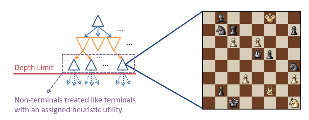Example of imperfect real-time heuristics.