Lecture 10: Constraint Satisfaction Problems - Backtracking and Filters

Note

Much of the content from these notes is taken directly or adapted from the notes of the same course taught by Dr. Andrew Forney available at forns.lmu.build.

Introduction

We’ll start this lecture by reflecting on the backtracking algorithm we discussed in the previous lecture. Recall the CSP with three variables we used as an example.

Question

Can you identify any ways to improve the backtracking algorithm applied to the CSP above (in terms of efficiency)?

Some possible improvements include:

• Some variable domains are too loose.
  • For example, constraint #2 implies that $R\ne 2$.
  • Constraint #3 implies that $T\ne 0$ and $S\ne 2$.
• The order in which we assign values to variables and the order in which we choose variables to assign to can matter.

Filtering

In this section we’ll address our first observation above: that some of the variables domains can be restricted based on the constraints.

Filtering is a technique for improving backtracking by reducing the domains of unassigned variables based on the constraints and assignments to other variables.

Filtering helps reduce the branching factor of the recursion tree during backtracking, making some large CSPs solvable in a reasonable amount of time.

Constraint Graphs and Consistency

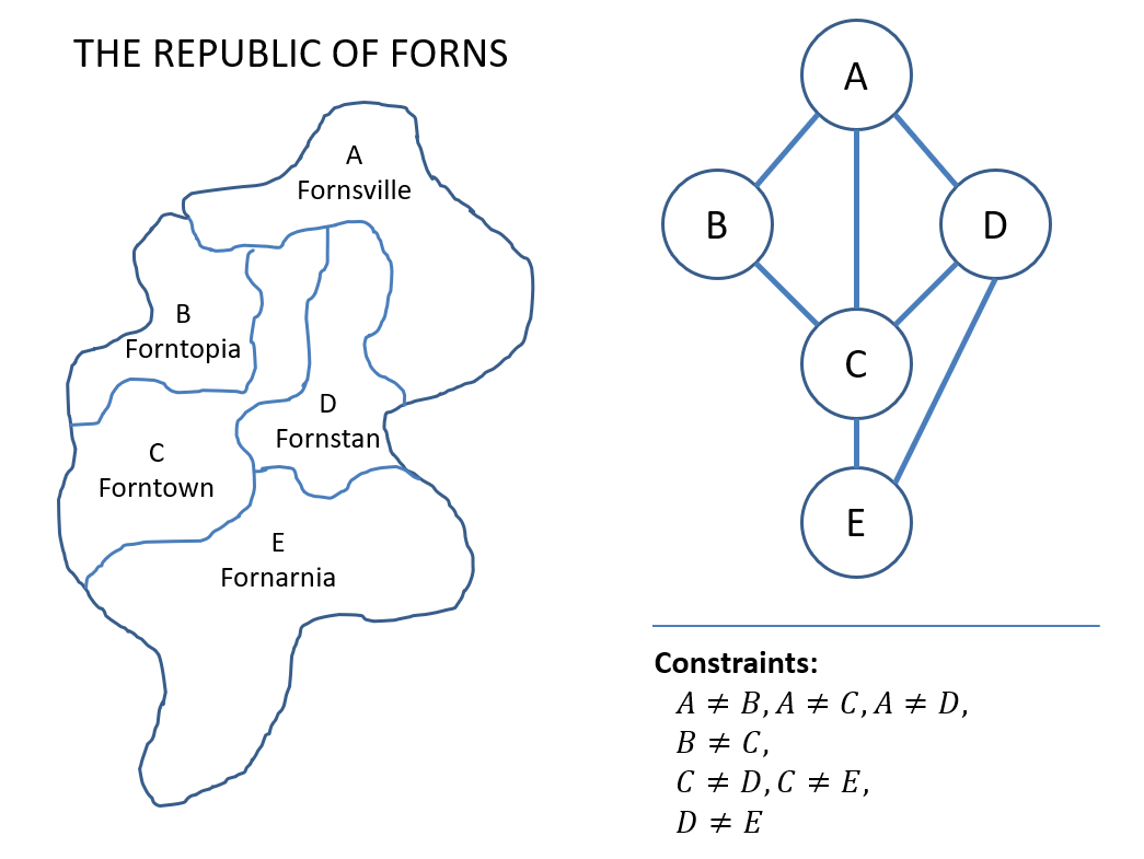
Earlier, when dealing with the Map Coloring problem, we created a graph of the adjacent nations.

Question

How might these kinds of graphs be useful with respect to filtering in other CSPs?

Constraint graphs allow us to determine which variables’ domains are dependent based on which variables are found in the same constraints.

In a constraint graph:

• Nodes are variables.
• Edges connect any two variables that appear in a constraint together.

Using these graphs, we can verify that, at any stage, the values in each variable’s domains are those that are still useful to consider.

Variable domains are said to be consistent when they contain only values that are potential candidates for a solution (subject to a specified granularity of consistency).

We’ll start with the simplest kind of consistency check: Node Consistency, which ensures that domains are consistent for any unary constraints pertaining to a particular node in the constraint graph. A unary constraint involves only a single variable.

For example, consider the CSP with two variables and different domains:

$$\begin{array}{rl}X& =\{A,B\}\\ D_A& =\{0,1,2\}\\ D_B& =\{0,1,2\}\\ C& =\{B<1,A\ne B\}\end{array}$$

In this example, the first constraint is unary and restricts the domain of $B$.

To enforce node consistency for node $B$: $D_B\leftarrow \{0\}$

Node $A$ is already node consistent: $D_A\leftarrow \{0,1,2\}$

After enforcing node consistency, we can further restrict the domain of $A$ by noting that since $B$ can only be 0 and $A\ne B$, $A$ cannot be 0.

This deduction was possible because we knew that $A$ and $B$ were connected in certain constraints and therefore adjacent in the constraint graph.

To check consistency between variables, we perform a new type of check: Arc Consistency, which ensures that domains are consistent for any binary constraints pertaining to any pairs of adjacent nodes in the constraint graph.

Consider a constraint graph in which two adjacent variables $A$ and $B$ are connected by an edge.

A directed arc is consistent if and only if for all values in the tail domain there is at least one value in the head domain that satisfies the arc’s constraint.

Values in the tail with no satisfying values in the head are removed from the tail domain.

Warning

A common misunderstanding is that we only prune values from the tail variable’s domain if any are inconsistent for a single arc.

See the example in the figure below for an illustration of how the domain of $A$ gets restricted due to arc consistency.

Recall our domains after enforcing node consistency are:

$$\begin{array}{rl}{D}_A& =\{0,1,2\}\\ D_B& =\{0\}\end{array}$$

In enforcing arc consistency $B\to A$, we find that there is at least one value in $D_A$ that satisfies the only value in $D_B$. Thus, we need not modify $D_B$.

In enforcing arc consistency $A\to B$, we find that there is no value in $D_B$ that satisfies the arc constraint for $A=0$. Therefore, we prune it from the domain of $A$:

$D_A\leftarrow \{1,2\}$

Note that checking for arc consistency does not perform the backtracking itself! Consider the following example:

$$\begin{array}{rl}X& =\{A,B\}\\ D_A& =\{0,1\}\\ D_B& =\{0,1\}\\ C& =\{A\ne B\}\end{array}$$

Question

Are $A$ and $B$ arc consistent in the above example?

Yes, each has at least one value in the other domain that can satisfy each of its values for the constraint $A\ne B$.

In summary, filtering can result in one of several outcomes:

• Filtering reduces a domain to the empty set: No solution to this CSP.
• Filtering reduces each domain to a single value: We have our solution.
• Filtering reduces each domain to some multitude of values: Still requires backtracking to find a solution.

Forward Checking

Consider a simplified Map Coloring problem with 3 colors and assignment order $[A,B,C,D,E,F]$. Suppose we’ve assigned $A=\text{Blu}$ and $B=\text{Red}$ (see figure below).

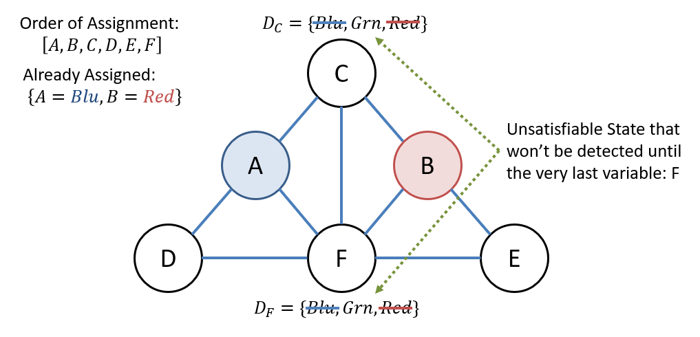
After assigning $A=\text{Blu}$ and $B=\text{Red}$, the only possible value for $C$ and $F$ is $\text{Grn}$.

Notice, however, that $C$ and $F$ are connected, and we won’t discover this conflict until we’ve assigned to every other variable!

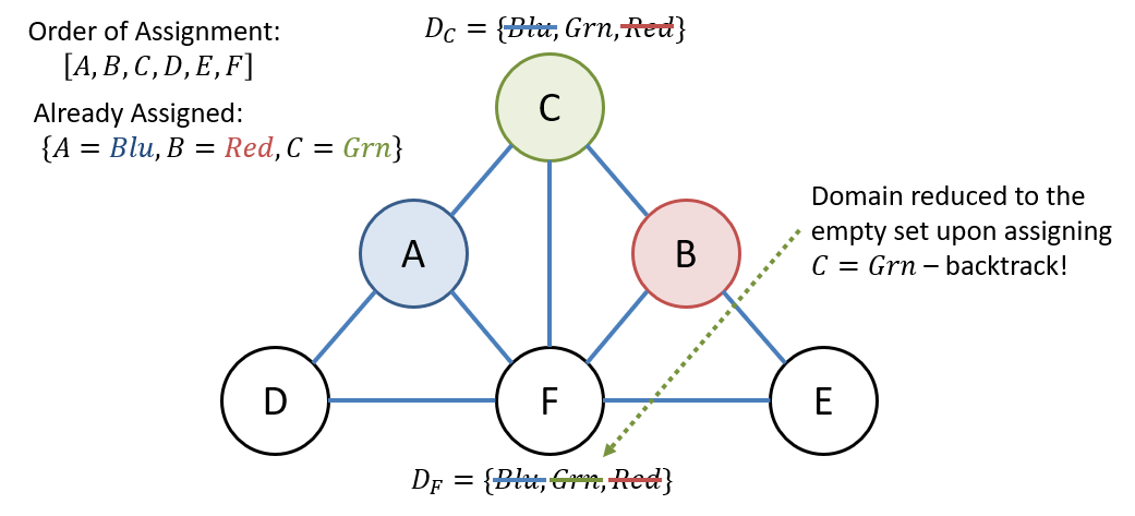
Forward Checking is a filtering technique deployed during backtracking that performs arc-consistency filtering between a newly assigned variable $X$ and its neighbors $\text{neighbors}(X)$.

In other words, during backtracking, if we assign a value to a variable in one of the partial states, forward checking restricts the domains of its neighbors that are yet to be assigned with respect to arc consistency.

This leads to an improvement in the backtracking efficiency because:

1. There are fewer values in domains to explore
2. We have an early backtracking condition if a variable’s domain is ever reduced to the empty set

Question

After assigning a value to what variable could we have detected the inevitable conflict in the example above?

After assigning to $B=\text{Red}$, we could have detected the conflict without needing to assign to $C$ to backtrack.

The idea is to propagate the domain restrictions to as many arcs as possible once an assignment is made.

Constraint Propagation

Constraint Propagation is a filtering technique in which any changes to domains made by arc consistency are recursively propagated to neighbors in the constraint graph.

The general idea is to re-check the neighbors of the modified domain in the constraint graph each time a change to a domain is made by arc consistency. Repeat this process until all arcs have been made consistent.

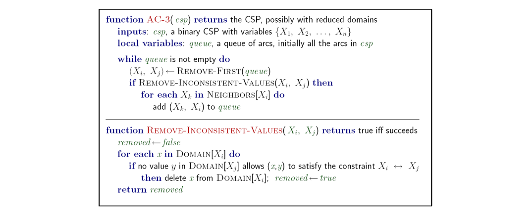
The AC-3 (arc-consistency, 3rd edition) Algorithm can be used for constraint propagation.

The steps of AC-3 are as follows:

1. Maintain a set of arcs (tail $\to$ head) to check for consistency, starting with all arcs in the set (referred to below as a queue but the actual data structure is a set).
2. While the set is not empty, pop an arc:
   • If it’s consistent, continue.
   • If it’s inconsistent, remove the offending values from the tail domain, then re-add all neighboring arcs that point to the tail.

See the figure below for the formal definition of the AC-3 algorithm.

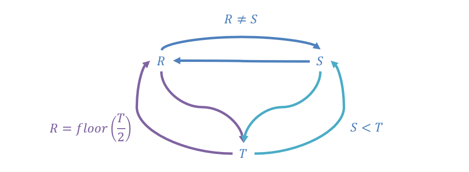
Consider our 3-variable example with $R,S,T$ and the constraints $R\ne S$, $R=\lfloor T/2\rfloor$, and $S<T$.

The arcs in the constraint graph are shown in the figure below.

Now, let’s trace the steps of AC-3 on this example to reduce the variable domains (see figure below).

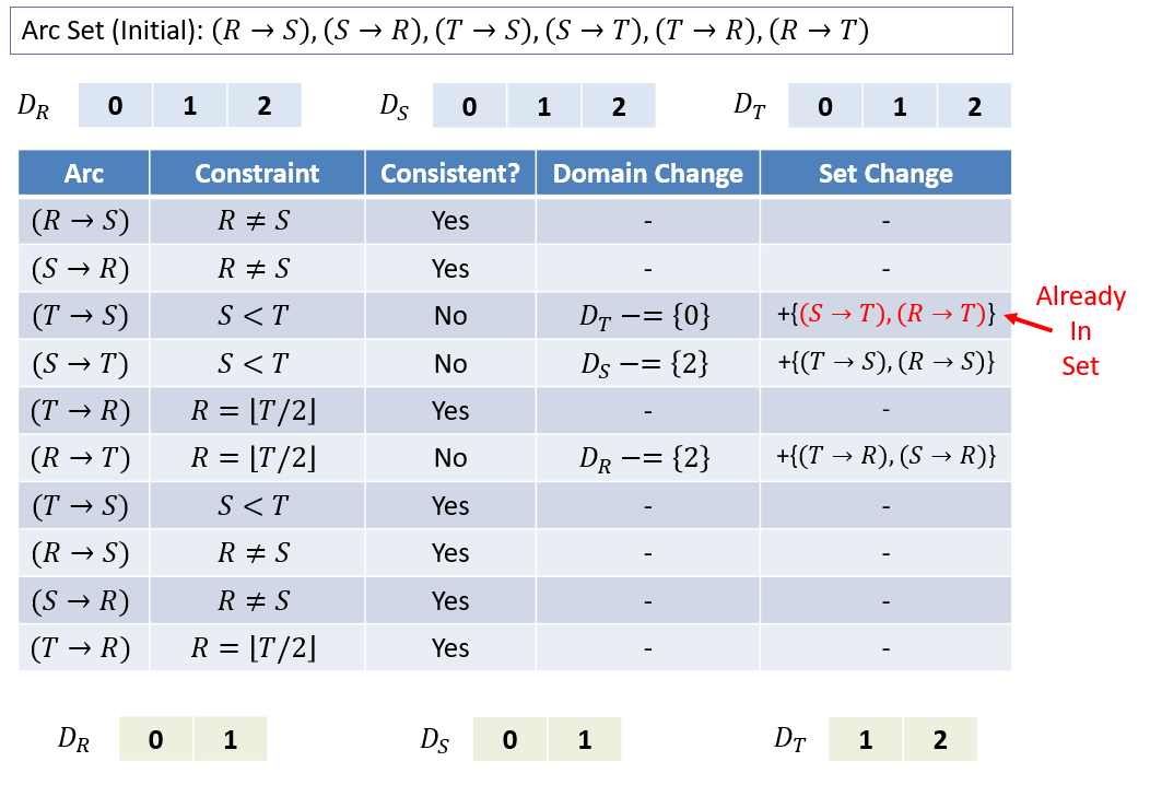
Warning

Note that in the example above, the queue additions ended up not being significant, but they might be in general.

We trimmed a value off of each domain, which (for large problems) can have a profound performance effect.