Lecture 1 - Uninformed Search

Note

Much of the content from these notes is taken directly or adapted from the notes of the same course taught by Dr. Andrew Forney available at forns.lmu.build.

Introduction

What is an algorithm? An algorithm is a step-by-step procedure for solving a problem. In other words, it is a sequence of instructions that describes how to solve a problem. In CMSI 2120, you learned about data structures and some algorithms that operate on them. In this course, we will shift our attention to studying different algorithm paradigms that can be used to solve problems.

What is a paradigm? A paradigm is a model or pattern that serves as a framework for solving problems. In this course, we will study several algorithm paradigms! With these, you will learn how to identify common patterns in problems and apply the appropriate algorithm to solve them.

Let’s start with a beginning example: Maze Path-finding (MP for short). Our agent starts at a given location in a grid-world maze and must find a path to a goal location. The agent can move in four directions: up, down, left, and right. The agent cannot move through walls, and the goal is to find the shortest path to the goal location.

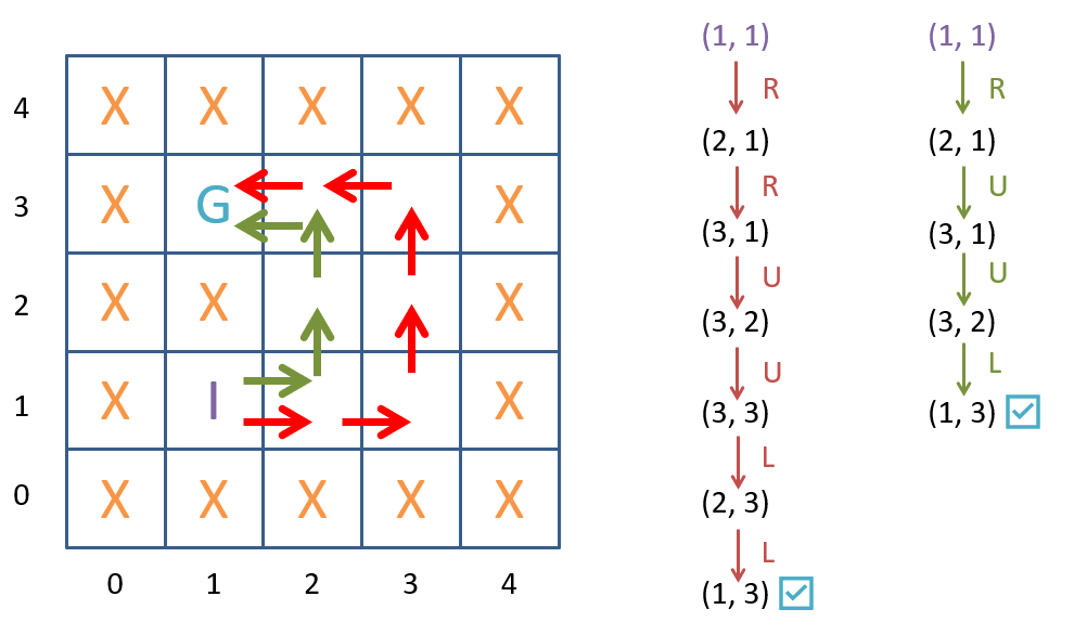A simple maze and two example solutions.

Observe in the figure above two (of the many) possible solutions to the maze. The first solution is the shortest path, while the second solution is longer. The goal of our agent is to find the shortest path to the goal location. The set of all possible solutions (paths) to the maze is called the search space. Now let’s see how we can formalize this problem and then look at some search strategies to solve it!

A General Formalization

We can formalize combinatorial search problems, problems that involve finding a solution in a large search space (like MP), as having the following five components:

1. Initial State: The starting configuration of the problem.
2. Goal State: The desired configuration of the problem.
3. Actions: The set of choices the agent can make to move from one state to another.
4. Transition Model: A description of how the state changes when an action is taken.
5. Cost: A function that assigns each transition a constant cost $c$.

Take a minute to think about how you would define these components for the MP problem, then confirm your answers with mine below:

1. Initial State: The agent’s starting location in the maze.
2. Goal State: The goal location in the maze.
3. Actions: The agent can move up, down, left, or right.
4. Transition Model: The agent moves to the new location when an action is taken.
5. Cost: The cost of moving from one location to another is 1.

Note that the way I’ve defined the problem, the cost is the same for all transitions. This is called a uniform cost problem.

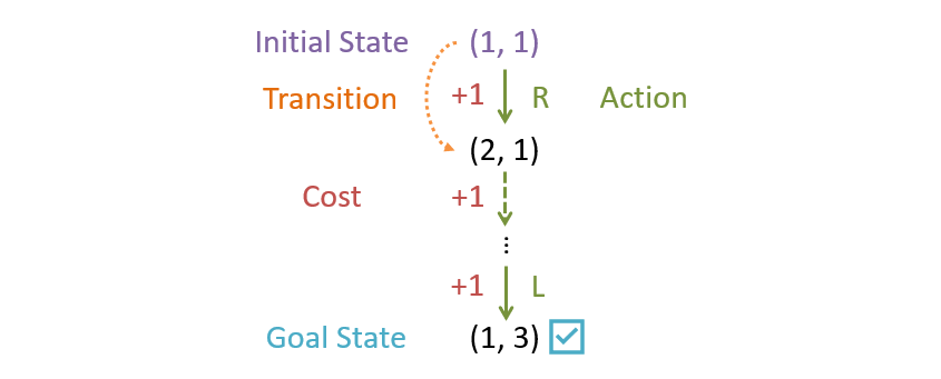A depiction of the components MP formalized as a search problem.

Question

What other problems can you think of that can be formalized as a combinatorial search problem?

Some examples of other problems that can be formalized as combinatorial search problems include:

• Solving a Rubik’s cube.
• Finding the shortest path in a road network.
• Types of planning where steps must be taken in a specific order (e.g., baking a pie or changing car oil).

Formalizing Search Strategies

Now that we’ve defined our problem, we need to find a way to solve it. We can do this by searching through the search space for a solution. For the MP problem, we need a systematic way to find the shortest path from the initial state to the goal state (hopefully without explicitly considering all paths since there are so many!).

Question

Can you think of an appropriate data structure to represent the search space for the MP problem?

One way to represent the search space is as a search tree. A search tree is a tree where each node represents a state in the search space, and the edges represent the actions that can be taken to move from one state to another. The root of the tree is the initial state, and the leaves are the goal states.

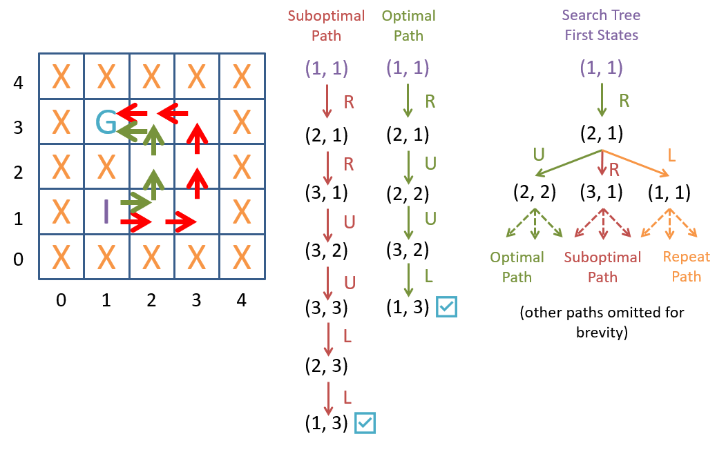A search tree for the MP problem.

A search strategy is a procedure for constructing and traversing a search tree to find a solution to a search problem. Because the search space can be very large or infinite (our MP problem has an infinite search space), we need to be strategic about how we construct and traverse the search tree. Clearly, we can’t construct the entire search tree up front since it would never finish! Instead, we will construct the search tree as we traverse it by keeping track of the frontier of the search tree, the set of nodes that we have yet to explore in a companion data structure.

1. Frontier Expansion: Remove a node from the frontier and add it as the next node to explore.

expandedNode = frontier.pop()

2. Frontier Generation: Add all possible next states from the current node to the frontier.

for a in actions(expandedNode):
    frontier.add(transition(expandedNode, a))

Each node in a search tree tracks:

1. The state the node represents.
2. The parent node that generated it (for creating the path to the solution).
3. The action that was taken to generate it (since there may be multiple ways to reach a state).
4. The cost of reaching the state (for non-uniform cost problems).

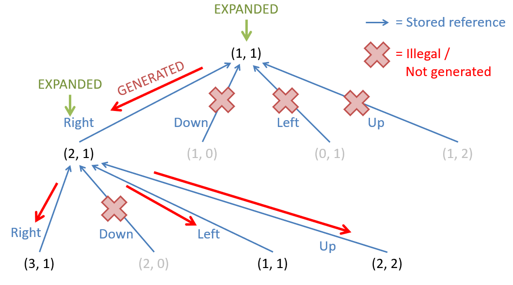Here is a search tree where we expand the root, generating its children (assuming each movement is legal), and then expand the child node corresponding to a taken “right” action.

Note in the figure above:

• The red arrows show the direction of node generation from parent to child (i.e., after expanding a parent, and concluding it is not the goal, we then generate the children).
• The blue arrows show the references that each child node remembers of its parent (important for remembering the path that led to it).
• Some nodes that would otherwise be generated are not because the action that would have generated them is illegal from the parent’s state (viz., those actions are ones that would run you into a wall!)
• Pausing the search tree construction at the image above, the leaf nodes $(3,1),(1,1),(2,2)$ would be the nodes stored in the frontier.

Now that we’ve decided how to generate the search tree, we need to decide how to traverse it!

Breadth-First Search

Breadth-First Search (BFS) is a search strategy that systematically explores the search tree by expanding the shallowest unexpanded node. To do this, BFS uses a FIFO queue as the frontier data structure. This ensures that nodes are expanded in the order they were generated.

Breadth-First Search on the search tree.

The figure above shows BFS on the search tree using the action precedence of: right, down, left, up. The nodes are expanded in the order they were generated, starting with the root node. BFS guarantees that the first solution found is the shortest path to the goal state.

Metrics of Optimality

When evaluating the performance of a search strategy, we may consider several metrics:

1. Completeness: A search strategy is complete if it is guaranteed to find a solution if one exists.
2. Optimality: A search strategy is optimal if it is guaranteed to find the shortest path to the goal state.
3. Time Complexity: An asymptotic measure of the number of steps required to find a solution.
4. Space Complexity: An asymptotic measure of the amount of memory required to find a solution.

Question

Is BFS complete?

Yes! BFS is complete because it will find a solution if one exists. This is because BFS systematically explores the search tree by expanding the shallowest unexpanded node.

Question

Is BFS optimal?

Yes, for a uniform cost problem, BFS is optimal because it guarantees that the first solution found is the shortest path to the goal state (the shallowest path in the search tree).

Question

What’s the worst-case asymptotic bound of memory/space required to store items in any List, Stack, Queue, Priority Queue, Map, or Set?

The worst-case asymptotic bound of memory/space required to store $n$ items in any of these data structures is $O(n)$.

Question

What is the time and space complexity of BFS?

To analyze the time and space complexity of BFS, we need to consider the size of the search tree. We can parameterize the size of the search tree by the depth of the shallowest solution $d$ and the maximum branching factor $b$ (see figure below).

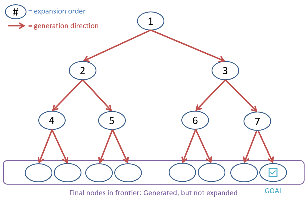The search tree for BFS with a branching factor of 2 and a depth of 3.

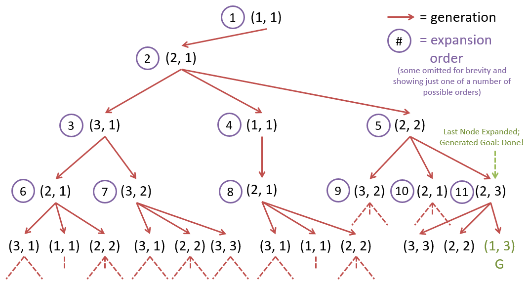
Let’s characterize the worst-case performance by considering the case when the goal state is the last to be expanded in the search tree (we assume that the algorithm terminates as soon as the goal state is generated — not expanded). See the table below for the number of nodes expanded, generated, and in memory at each level of the search tree.

Tree Level	Nodes Expanded	Nodes Generated	Nodes in Memory
0	$b^0=1$	$b^1=2$	$b^0+b^1=3$
1	$b^1=2$	$b^2=4$	$b^0+b^1+b^2=7$
2	$b^2=4$	$b^3=8$	$b^0+b^1+b^2+b^3=15$
⋮	⋮	⋮	⋮
$d-1$	$b^{d-1}$	$b^d$	$b^0+b^1+\cdots +b^d$

The number of nodes expanded, generated, and in memory at each level of the search tree.

Thus, in level $d$ (when the goal state is expanded in the last step), the total number of nodes that have been expanded is $b^0+b^1+\cdots +b^{d-1}=O(b^d)$ and the total number of nodes that have been generated is $b^0+b^1+\cdots +b^d=O(b^{d+1})$. Thus, the time complexity of BFS is $O(b^d)$ (remember that with asymptotic notation, we drop the lower-order terms and constants). The total number of nodes in memory by the time the goal state is expanded is $b^0+b^1+\cdots +b^d=O(b^d)$. Thus, the space complexity of BFS is $O(b^d)$.

Graph Search

An observant student might look at the last search tree and remark: some states are repeated in expansion! This is, in fact, the main issue with the search tree model: it does not account for repeated states.

Question

How can we account for repeated states in our search tree?

A search graph is a search tree that accounts for repeated states by not expanding a state that has already been expanded. We can use another auxiliary data structure (a set) to keep track of the states that have been expanded. We’ll call this set the graveyard.

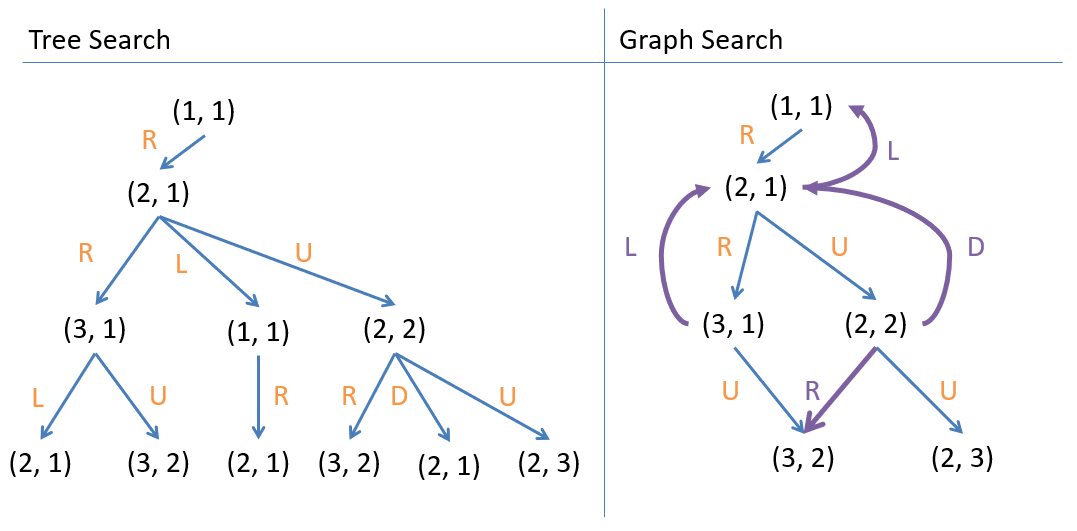Graph Search on the search tree.

The figure above shows Graph Search on the search tree. The purple edges represent transitions to states that have already been expanded and are not expanded again.

Tip

Record-keeping of past effort to avoid repeating effort in the future is a form of a more general paradigm known as memoization / caching that we’ll explore more later.

Depth-First Search

Naturally, if BFS is an uninformed search strategy, we should examine the merits of Depth-First Search as well! Depth-First Search (DFS) is a search strategy that systematically explores the search tree by expanding the deepest unexpanded node. To do this, DFS uses a LIFO stack as the frontier data structure.

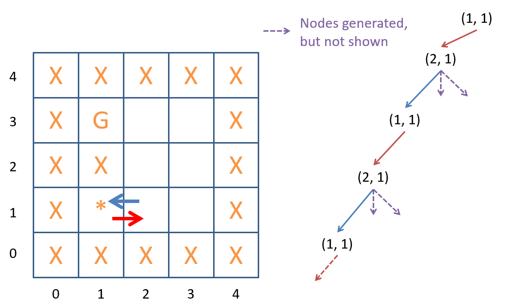An unsuccessful Depth-First Search on the search tree.

Observe, however, that DFS can get stuck in an endless expansion loop if the search tree is infinite (see figure above)! The example in the figure shows DFS getting stuck because the agent keeps going back and forth between the same two states. This begs the question, then: can we use memoization to avoid this issue? Maybe, but we would need to be careful: unlike in the case of breadth-first search, the first solution found by depth-first search is not guaranteed to be the shortest path to the goal state (see figure below).

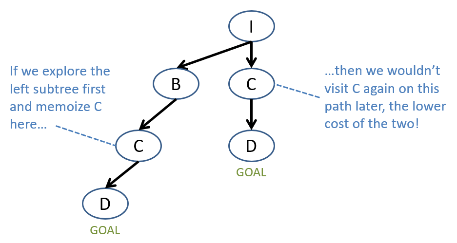Memoization can help avoid infinite loops in DFS, but may not guarantee optimality if you’re not careful!

There is an alternative approach to DFS that can help avoid the infinite loop issue and has some other benefits as well.

Question

If we knew the depth of the shallowest goal node, what could we potentially limit to satisfy both of the above?

We could limit the depth of the search tree to the depth of the shallowest goal node. This approach is called Depth-Limited Search. Using depth-limited search, suppose we generated the same search tree as with the BFS example, though (for readability) now add nodes to our Stack frontier in right-to-left order ($b=2,d=3,m=3$).

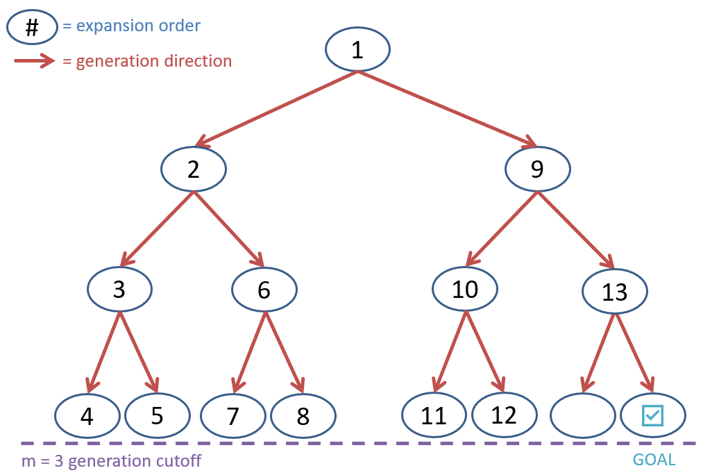Depth-Limited Search on the search tree.

Some comments on the figure above:

• We’re showing the nodes at the cutoff depth as being expanded to demonstrate the DFS frontier ordering, even though they do not generate any children.
• The final two nodes generated (level 3, far right) are not expanded because our goal test is still being performed at generation, not expansion.
• This might look like it’s doing more work than the BFS equivalent, but note that we’ve generated the same number of nodes!

Because we generate the same number of nodes as BFS, we see that the time complexity of depth-limited search is the same, just at our depth cutoff of $m$, giving us $O(b^m)$.

So what’s the benefit of Depth-Limited Search over BFS that I mentioned earlier?

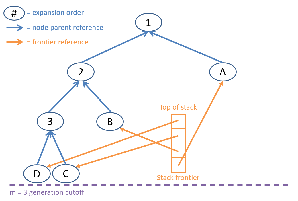The memory usage of Depth-Limited Search.

The figure above gives us a hint: how is the memory usage of Depth-Limited Search different from BFS? To answer this question, let’s analyze the time and space complexity of Depth-Limited Search using the same parameters as before: the depth of the shallowest solution $d$ and the maximum branching factor $b$.

Question

What is the maximum size of the frontier in Depth-Limited Search?

The maximum size of the frontier in Depth-Limited Search is $O(bm)$, where $m$ is the depth limit! This is because the frontier will never contain more than $b$ nodes at any level of the search tree, and we only need to keep track of the nodes at the current depth and the nodes at the previous depth (to backtrack). This is a significant improvement over BFS, which can require storing $O(b^{d+1})$ nodes in memory!

Iterative Deepening Depth-First Search

Question

What is the main drawback of Depth-Limited Search?

We don’t know the depth of the shallowest solution in advance, so we have to guess a depth limit $m$. If $m$ is too small, we might miss the goal state. If $m$ is too large, we might waste time exploring nodes that are not on the path to the goal state. To address this issue, we can use an approach called Iterative Deepening Depth-First Search.

Iterative Deepening Depth-First Search (IDDFS) performs a series of depth-limited searches with increasing depth limits until the goal state is found.

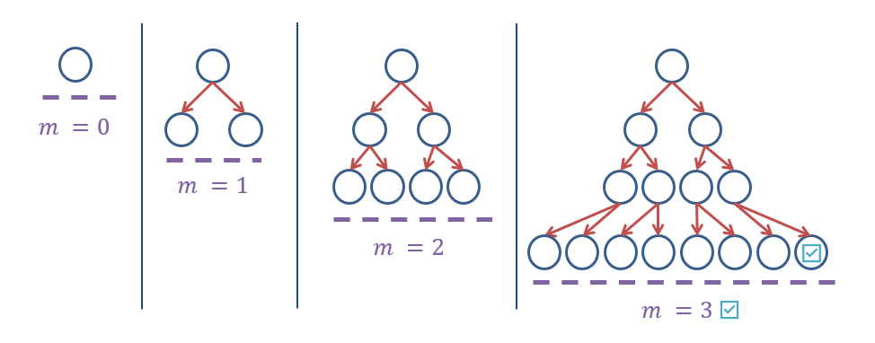Iterative Deepening Depth-First Search on the search tree.

Warning

Observe that a new search tree is generated for each depth limit in IDDFS!

Question

Will IDDFS have the same time complexity as BFS? Why or why not?

Yes! The largest depth limit in IDDFS is the depth of the shallowest solution $d$ and has a time complexity of $O(b^d)$. This complexity dominates (asymptotically) the time complexity of the shallower searches, so the overall time complexity of IDDFS is $O(b^d)$.

Question

Will IDDFS have the same space complexity as BFS? Why or why not?

No! IDDFS will have a space complexity of $O(bd)$, where $d$ is the depth of the shallowest solution. IDDFS thus preserves the completeness enjoyed by BFS while gaining the space-saving features of DFS, for the small overhead of having to repeat earlier parts of the search. As such, BFS has a smaller constant-of-proportionality due to the IDDFS overhead of exploring smaller models, but has the same asymptotic runtime.